SAS Programming: Dive into the world of powerful data analysis! From its humble beginnings, SAS has evolved into a leading statistical software package used across industries. This guide will walk you through the core concepts, from importing data and cleaning it up to performing complex statistical analyses and creating stunning visualizations. We’ll cover everything from the basics of SAS syntax to advanced procedures, ensuring you’re equipped to tackle any data challenge that comes your way.
Table of Contents
We’ll explore the different types of SAS datasets, the nuances of data manipulation, and the power of SAS procedures like PROC MEANS, PROC FREQ, and PROC REG. You’ll learn how to write efficient and effective SAS programs, handle errors, and even delve into the world of SAS macros and big data analytics. Get ready to unlock the potential of SAS and transform raw data into actionable insights!
Introduction to SAS Programming
SAS, or Statistical Analysis System, is a powerful and widely used software suite for data management, advanced analytics, and business intelligence. It’s been a staple in the data science world for decades, evolving from its humble beginnings to become a comprehensive platform for handling everything from simple data cleaning to complex statistical modeling. Understanding its history and components is key to unlocking its potential.
A Brief History of SAS
SAS originated in the 1960s at North Carolina State University as a tool for statistical analysis. Early versions focused on agricultural research, but its capabilities quickly expanded. Over the years, SAS has undergone significant development, incorporating new features like data mining, business intelligence tools, and advanced analytics techniques. This evolution reflects the growing demand for more sophisticated data analysis in various fields, including healthcare, finance, and marketing.
Today, SAS is a global leader in analytics software, used by organizations of all sizes worldwide.
Core Components of the SAS System
The SAS System is not just a single program; it’s a suite of integrated software products. Key components include SAS Studio, a user-friendly interface for writing and running SAS code; SAS Base, providing fundamental data manipulation and statistical procedures; and various add-on modules, such as SAS/STAT for advanced statistical analysis, SAS/GRAPH for data visualization, and SAS/IML for matrix programming.
These components work together seamlessly, allowing users to perform a wide range of data-related tasks within a unified environment. The modular design allows organizations to tailor their SAS implementation to their specific needs and budget.
SAS Data Set Types
SAS data sets are the foundation upon which all SAS analyses are built. They are not simply files; they’re structured collections of data organized in a specific format. The most common type is the SAS data set, which is a tabular structure similar to a spreadsheet, with rows representing observations and columns representing variables. However, SAS also supports other data structures, including:
- SAS Data Sets (the standard): These are the workhorses of SAS, containing both data and metadata (information about the data itself). They are efficient for storage and processing within the SAS system.
- External Files: SAS can import and export data from various external sources like CSV, Excel, and databases. This allows for seamless integration with other systems.
- Temporary SAS Data Sets: These are created during a SAS session but are automatically deleted when the session ends. They are useful for intermediate steps in data processing, preventing the accumulation of unnecessary files.
Understanding these different data set types is crucial for efficient data management and analysis within the SAS environment. Choosing the right type depends on the specific needs of the project and the intended use of the data.
Data Manipulation in SAS
Data manipulation is the heart of any SAS project. Once you’ve imported your data, the real work begins – cleaning, transforming, and preparing it for analysis. This section covers importing data from various sources and then dives into essential data cleaning techniques, focusing on handling missing values and outliers.
Importing Data into SAS
SAS offers several ways to import data, each suited to different file types and scenarios. `PROC IMPORT` provides a straightforward method for importing data from common file formats like Excel spreadsheets and CSV files. `PROC SQL` offers a more powerful and flexible approach, especially when dealing with complex data sources or requiring data manipulation during the import process.
Using PROC IMPORT for Data Import
`PROC IMPORT` is your go-to for quick and easy data imports. For example, to import an Excel file named “mydata.xlsx” into a SAS dataset named “sasdata”, you’d use the following code: proc import datafile="mydata.xlsx" out=sasdata dbms=xlsx replace; getnames=yes;run;This code specifies the file path, the output dataset name, the database management system (DBMS) type, and indicates that existing datasets with the same name should be replaced.
The `getnames=yes;` option automatically assigns variable names from the Excel file’s header row. Similar syntax applies for CSV files, simply changing the `dbms` option to `csv`.
Using PROC SQL for Data Import
`PROC SQL` provides a more versatile method, allowing for data manipulation during the import process. For instance, you could import data from a text file, filtering rows based on specific criteria. This requires specifying the file’s structure using the `INTO` statement and applying `WHERE` clauses for filtering. proc sql; create table sasdata as select from file 'mydata.txt' delimiter=',' dbms=csv where column1 > 10;quit;This example imports data from “mydata.txt,” using a comma as the delimiter, and only includes rows where the value in `column1` is greater than 10.
Data Cleaning Techniques
Data cleaning is crucial for accurate analysis. Common techniques include handling missing values, identifying and addressing outliers, and correcting inconsistencies in data formats. SAS provides a wealth of functions and procedures to facilitate this process.
Handling Missing Values
Missing values are a common problem in datasets. SAS represents missing values with a period (.). Several approaches exist for handling them, including imputation (replacing missing values with estimated values) and exclusion (removing observations with missing values). The `PROC MI` procedure offers various imputation methods. Simple imputation methods can be done with SAS functions such as `IF-THEN-ELSE` statements to replace missing values with a specific value (e.g., the mean, median, or a designated value).
Identifying and Handling Outliers
Outliers are data points that significantly deviate from the rest of the data. They can skew results and distort analyses. Methods for detecting outliers include visual inspection (using histograms or box plots), and statistical methods such as calculating z-scores. Outliers can be handled by removing them, transforming the data (e.g., using logarithmic transformation), or using robust statistical methods less sensitive to outliers.
Example SAS Program for Missing Values and Outliers
This program demonstrates handling missing values and outliers using simple imputation and z-score based outlier detection. Note that this is a simplified example and more sophisticated techniques may be necessary for complex datasets. data cleaned_data; set original_data; if age=. then age = mean(age); /*Imputes missing age values with the mean age*/ z_score = (weight - mean(weight))/std(weight); /*Calculates z-scores for weight*/ if abs(z_score) > 3 then delete; /*Removes outliers (z-score >3 or <-3)*/
run;
This code first imputes missing age values with the mean age. Then, it calculates the z-scores for the weight variable. Finally, it removes observations where the absolute z-score for weight is greater than 3, effectively removing outliers based on a commonly used threshold.
Remember to replace `original_data` with your actual dataset name.
SAS Data Structures

Okay, so we've covered the basics of SAS programming and data manipulation. Now let's dive into the heart of how SAS actually
stores* your data
its data structures. Understanding these is crucial for efficient and effective SAS programming. Think of it like understanding the blueprint of a house before you start building – you need to know the foundation!
SAS datasets are fundamentally tabular. They're organized into rows and columns, just like a spreadsheet. Each row represents an observation (like a single person in a survey), and each column represents a variable (like age, income, or favorite color). Variables hold the data for each observation, and they have a specific data type (numeric, character, etc.). This structure makes it incredibly easy to work with large datasets and perform complex analyses.
SAS Datasets
SAS datasets are the workhorses of SAS. They are stored in a proprietary format (.sas7bdat) and are optimized for SAS's processing engine. They can hold both numeric and character data, along with metadata (information about the data itself, like variable names and types). Think of them as the primary storage container for your data within the SAS environment.
You create them using the DATA step, and they're the basis for most SAS procedures.
SAS Views
Unlike datasets, SAS views don't actually store data. Instead, they're essentially saved queries. They define how to access data from one or more underlying datasets. They're a powerful tool for creating customized subsets of data or combining data from different sources without having to physically copy and create a new dataset. This saves storage space and processing time, especially when dealing with huge datasets.
Think of them as a "virtual table" – they only exist as a definition, not as a separate data file.
Manipulating Data Structures: A SAS Program Example
Let's illustrate this with a simple example. We'll create a dataset, then create a view based on that dataset.
/* Create a sample dataset
-/
data my_data;
  input name $ age height;
  datalines;
John 25 72
Jane 30 68
Mike 28 70
;
run;

/* Create a view showing only people over 28
-/
proc sql;
  create view older_people as
  select
-
  from my_data
  where age > 28;
quit;

/* Print the view
-/
proc print data=older_people;
run;

/* Print the original dataset to show the difference
-/
proc print data=my_data;
run;
This program first creates a dataset called `my_data` containing names, ages, and heights. Then, it creates a view `older_people` that only includes individuals older than 28. Finally, it prints both the view and the original dataset to demonstrate how the view only displays a subset of the original data without modifying the original dataset itself. This highlights the difference between a SAS dataset (which stores data) and a SAS view (which defines how to access data).
Statistical Analysis with SAS
Okay, so we've covered the basics of SAS programming, data manipulation, and data structures. Now let's dive into the fun stuff: using SAS for statistical analysis! SAS offers a powerful suite of procedures for tackling various statistical problems, and we'll explore some of the most commonly used ones. We'll focus on descriptive statistics, frequency distributions, linear regression, and hypothesis testing (t-tests and ANOVA).
PROC MEANS for Descriptive Statistics
PROC MEANS is your go-to procedure for calculating basic descriptive statistics like mean, standard deviation, median, minimum, and maximum. It's incredibly versatile and lets you easily summarize your data across different variables and groups. For example, let's say you have a dataset named 'grades' with variables 'studentID', 'exam1', and 'exam2'. To get descriptive statistics for both exams, you'd use the following code:
proc means data=grades mean std median min max;

  var exam1 exam2;

run;
This code will output a table showing the mean, standard deviation, median, minimum, and maximum scores for both 'exam1' and 'exam2'. You can customize this further by adding options like `n` (to get the number of observations) or `clm` (for confidence limits).
PROC FREQ for Frequency Distributions
PROC FREQ is perfect for examining the distribution of categorical variables. It generates frequency tables, percentages, and cumulative frequencies, providing insights into the proportions of different categories within your data. Imagine you have a dataset 'survey' with a variable 'favoriteColor'. To see how many people chose each color, you'd use:
proc freq data=survey;

  tables favoriteColor;

run;
This produces a frequency table showing the count and percentage of each color. You can add options like `chisq` to perform a chi-square test of independence if you have multiple categorical variables.
PROC REG for Linear Regression Analysis
PROC REG is a workhorse for linear regression. It helps you model the relationship between a dependent variable and one or more independent variables. Let's say you want to predict 'housePrice' based on 'size' and 'location' (coded numerically). Your code might look like this:
proc reg data=housing;

  model housePrice = size location;

run;
PROC REG will output the regression coefficients, R-squared, F-statistic, and other relevant statistics to assess the model's fit and significance. You can further explore diagnostics like residual plots to check the assumptions of linear regression.
T-tests and ANOVA using SAS Procedures
For comparing means between groups, SAS offers several procedures. T-tests are used for comparing the means of two groups, while ANOVA (Analysis of Variance) extends this to multiple groups. Let's assume we have a dataset 'experiment' with a variable 'treatment' (with levels A and B) and a response variable 'growth'.
To perform a t-test:
proc ttest data=experiment;

  class treatment;

  var growth;

run;
For a one-way ANOVA with multiple treatment levels (say, A, B, and C):
proc glm data=experiment;

  class treatment;

  model growth = treatment;

run;
Both procedures will provide p-values to assess the statistical significance of the difference in means.
| Test | Procedure | Purpose | Example Data |
|---|---|---|---|
| Independent Samples t-test | PROC TTEST | Compare means of two independent groups | Comparing exam scores between two different classes |
| Paired Samples t-test | PROC TTEST | Compare means of two related groups | Comparing pre- and post-treatment scores for the same individuals |
| One-way ANOVA | PROC GLM | Compare means of three or more independent groups | Comparing plant growth under different fertilizer treatments |
| Two-way ANOVA | PROC GLM | Compare means with two or more factors | Analyzing the effects of fertilizer and watering frequency on plant growth |
SAS Programming Syntax and Control Flow
Okay, so we've covered the basics of SAS – data manipulation, structures, and even some stats. Now it's time to dive into the nitty-gritty of actually
-writing* SAS programs. This means understanding the syntax and how to control the flow of your code, making it do exactly what you want. Think of it as learning the grammar and sentence structure of the SAS language.
SAS programs are built using statements, each ending with a semicolon (;). These statements can be DATA steps (used for data manipulation) or PROC steps (used for procedures like statistical analysis). Whitespace (spaces, tabs, and newlines) generally doesn't affect the code's execution, but proper indentation makes your code much more readable – and believe me, you'll thank yourself later when debugging.
IF-THEN-ELSE Statements
IF-THEN-ELSE statements are the workhorses of conditional logic in SAS. They allow your program to make decisions based on whether a condition is true or false. The basic structure is straightforward: IF condition THEN statement; ELSE statement;. The `ELSE` part is optional; if the condition is false and there's no `ELSE`, nothing happens. Conditions use comparison operators like = (equals), ≠ (not equals), > (greater than), < (less than), ≥ (greater than or equal to), and ≤ (less than or equal to).
For example, let's say you have a dataset with a variable called 'Age'.
You might use an IF-THEN-ELSE statement to categorize individuals as "Adult" or "Minor":
data age_categories; set original_dataset; if Age >= 18 then Adult_Minor = 'Adult'; else Adult_Minor = 'Minor';run;
This code creates a new variable, 'Adult_Minor', assigning 'Adult' if 'Age' is 18 or greater, and 'Minor' otherwise.
DO Loops, Sas programming
DO loops are used for repetitive tasks. They execute a block of code a specified number of times or until a condition is met. A simple DO loop looks like this: DO i = 1 TO 10; statement; END;. This loop will execute the `statement` ten times, with the variable `i` incrementing from 1 to 10 in each iteration. You can also use a `DO WHILE` loop, which continues as long as a condition is true.
For instance, to calculate the sum of numbers from 1 to 100:
data sum_numbers; sum = 0; do i = 1 to 100; sum = sum + i; end;run;
Nested Loops and Conditional Statements
Combining DO loops and IF-THEN-ELSE statements allows for complex logic. Nested loops involve placing one loop inside another. This is useful when you need to iterate over multiple dimensions of data.
Let's create a program that simulates a simple game of tic-tac-toe, illustrating nested loops and conditional statements:
data tictactoe; array board[9] _temporary_ (0 0 0 0 0 0 0 0 0); /* Initialize the board - / do i = 1 to 9; /*Outer loop iterates through each turn*/ do while (board[i] = 0); /*Inner loop continues until an empty spot is found*/ /*Simulate player input - replace with actual game logic*/ board[i] = 1; /*Player 1 takes the spot*/ put i= board[i]=; leave; end; end;run;
This code initializes a 9-element array representing the tic-tac-toe board. The outer loop simulates each turn. The inner loop finds an empty spot (represented by 0) and places a marker (1 for Player 1 in this simplified example). This is a very basic example; a full tic-tac-toe game would require significantly more logic to handle player turns, win conditions, and more.
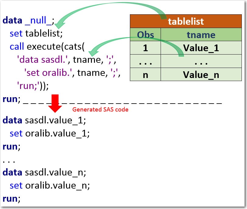
Working with Macros in SAS: Sas Programming
SAS macros are a powerful tool for automating repetitive tasks and creating more efficient and reusable code. They essentially allow you to write code that writes code, significantly reducing redundancy and improving maintainability, especially in large or complex projects. Think of them as mini-programs within your larger SAS program.
Macro Definition and Invocation
Macros are defined using the `%macro` statement and invoked using the `%mend` statement. The code between these statements constitutes the macro body. Once defined, you can call the macro multiple times within your program, passing different arguments each time. This is incredibly useful for tasks like generating reports with varying parameters or performing the same analysis on multiple datasets.
For example, a simple macro to print a message:```sas%macro print_message(message); put &message;%mend print_message;%print_message(Hello, world!);```This macro, `print_message`, takes a single argument, `message`, and uses the `put` statement to print its value to the log. Invoking `%print_message(Hello, world!)` will print "Hello, world!" to the SAS log.
So, SAS programming is killer for data analysis, right? But sometimes you need a simpler database for smaller projects, and that's where something like microsoft access comes in handy. Then, once you've cleaned and prepped your data in Access, you can easily import it back into SAS for more in-depth analysis and reporting.
Macro Variables
Macro variables are variables that hold text values within a macro. They're created using the `%let` statement. These variables are resolved (their values are substituted) during macro execution. They are essential for passing dynamic values into macros. For instance:```sas%let my_dataset = sashelp.cars;proc print data=&my_dataset;run;```Here, `%let my_dataset = sashelp.cars;` creates a macro variable named `my_dataset` and assigns it the value `sashelp.cars`.
The `proc print` statement then uses this macro variable to specify the dataset to be printed. Changing the value of `my_dataset` changes which dataset is printed without modifying the `proc print` statement itself.
Macro Functions
SAS provides several built-in macro functions that perform specific operations on macro variables or text strings. These functions are invaluable for manipulating text and creating more flexible macros. For example, `%sysfunc(upcase(...))` converts a string to uppercase, and `%sysfunc(scan(...,...,...))` extracts a specific word from a string.```sas%let my_string = Hello World;%put %sysfunc(upcase(&my_string)); /* Prints HELLO WORLD - /%put %sysfunc(scan(&my_string,2)); /* Prints World - /```These functions allow for dynamic text manipulation within your macros, enhancing their adaptability.
Automating a Repetitive Task with a Macro
Let's create a macro to generate summary statistics for multiple variables in a dataset. This task, if done manually, would require writing repetitive `proc means` statements. Our macro will automate this:```sas%macro generate_summary_stats(dataset, vars); proc means data=&dataset n mean std min max; var &vars; run;%mend generate_summary_stats;%generate_summary_stats(sashelp.cars, mpg weight);```This macro, `generate_summary_stats`, takes the dataset name and a list of variables as arguments.
It then uses `proc means` to generate summary statistics for the specified variables. This eliminates the need to write separate `proc means` statements for each variable, making the code much more concise and easier to maintain. Adding more variables only requires updating the `vars` argument in the macro call.
Advanced SAS Procedures
Okay, so we've covered the basics of SAS programming. Now let's dive into some of the more powerful and specialized procedures that SAS offers. These procedures allow for more complex data manipulation and statistical analysis, opening up a whole new world of possibilities for your data-driven projects. We'll explore PROC SQL, PROC PHREG, and PROC GLM, highlighting their strengths and weaknesses.
PROC SQL for Advanced Data Manipulation
PROC SQL is essentially SAS's way of incorporating SQL functionality. This is incredibly useful because it allows you to leverage the power and flexibility of SQL for data manipulation directly within your SAS environment. You can perform complex joins, subqueries, and aggregations with relative ease. For instance, imagine you have two datasets: one with customer information and another with their purchase history.
Using PROC SQL, you can easily join these datasets to create a single dataset containing all the relevant information for each customer. This is far more efficient than using SAS's data step for such complex operations. Here’s a simple example of joining two tables: PROC SQL; CREATE TABLE customer_purchases AS SELECT c.customer_id, c.customer_name, p.product_id, p.purchase_date FROM customer_info AS c JOIN purchase_history AS p ON c.customer_id = p.customer_id;QUIT;This code joins the `customer_info` and `purchase_history` tables based on the `customer_id` and creates a new table called `customer_purchases` containing the combined data.
You can extend this with `WHERE` clauses to filter data, `GROUP BY` to aggregate data, and various other SQL functions to perform even more sophisticated manipulations.
PROC PHREG for Survival Analysis
PROC PHREG is a lifesaver when you're dealing with time-to-event data. This type of data is common in fields like medicine (time until patient death or recovery), engineering (time until equipment failure), and finance (time until loan default). PROC PHREG allows you to fit proportional hazards models, which are used to estimate the probability of an event occurring at a given time, considering various factors.
For example, in a clinical trial, you might use PROC PHREG to model the time until a patient experiences a relapse, taking into account factors like treatment type and age. The output will provide hazard ratios, which show the relative risk of an event occurring based on different predictor variables. The underlying mathematics is a bit intense, involving hazard functions and survival functions, but PROC PHREG handles the heavy lifting, allowing you to focus on the interpretation of the results.
A typical PROC PHREG call might look something like this (simplified for clarity): PROC PHREG DATA=clinical_trial; MODEL time_to_relapse*status(0) = treatment_type age;RUN;Here, `time_to_relapse` represents the time until relapse, `status` indicates whether a relapse occurred (1) or the patient was censored (0, meaning the event didn't occur during the observation period), `treatment_type` is a categorical variable, and `age` is a continuous variable.
PROC GLM for Generalized Linear Models
PROC GLM is your go-to procedure for fitting generalized linear models (GLMs). GLMs are a powerful extension of ordinary least squares regression, allowing you to model various types of response variables, including binary (0/1), count data (e.g., number of accidents), and even survival data (though PROC PHREG is usually preferred for survival analysis). PROC GLM allows you to specify different link functions and error distributions to fit the model to the specific characteristics of your data.
For example, you might use a logistic regression (a type of GLM) to predict the probability of a customer churning based on factors like usage frequency and customer service interactions. Or, you could use a Poisson regression (another type of GLM) to model the number of car accidents at an intersection based on traffic volume and weather conditions.
The flexibility of PROC GLM is a significant advantage.
Strengths and Weaknesses of Advanced Procedures
Choosing the right advanced procedure depends heavily on your specific needs. PROC SQL excels in data manipulation and is relatively easy to learn if you have some SQL experience. However, it might not be the most efficient for extremely large datasets. PROC PHREG is specifically designed for survival analysis and provides detailed output for interpreting the results. However, it's less versatile than PROC GLM.
PROC GLM is incredibly versatile but can be more complex to use, requiring a good understanding of statistical modeling concepts. Each procedure has its strengths and weaknesses, making it crucial to choose the one that best suits the task at hand.
Error Handling and Debugging in SAS

So, you've written some SAS code, and it's... not working. Don't worry, it happens to the best of us! This section dives into the common pitfalls and powerful tools available to track down and squash those pesky SAS bugs. Mastering debugging is crucial for efficient SAS programming.
SAS programming, while powerful, can throw some curveballs. Understanding common error types and effective debugging strategies is essential for efficient and reliable code. This section will equip you with the tools to tackle these challenges head-on.
Common SAS Errors
Common SAS errors range from simple syntax mistakes to more complex logical errors. Identifying the error type is the first step toward a solution. Let's look at some examples. Syntax errors, such as misspelled s or incorrect punctuation, are often flagged by the SAS compiler. These are usually easy to spot.
More challenging are logical errors, where the code runs without error messages, but produces incorrect results. These require careful examination of the code logic and data. Finally, data errors—such as missing values or inconsistencies in data—can cause unexpected results. Understanding the different error types is crucial for effective debugging.
Debugging Techniques
Effective debugging involves a systematic approach. The SAS log is your best friend. It provides detailed information about the execution of your program, including error messages, warnings, and notes. Carefully examining the log often reveals the source of the problem. Another useful technique is the use of the `PUT` statement.
This allows you to print the values of variables at various points in your program, helping you track their values and identify unexpected behavior. Step-by-step execution, often called tracing, allows you to manually walk through the code line by line, observing the program's flow and variable changes. This is particularly helpful for identifying logical errors. Finally, using breakpoints within your code can pause execution at a specific point, allowing for detailed inspection of the program's state.
Using the SAS Log for Error Identification
The SAS log is a crucial tool. For example, imagine you have a simple data step with a syntax error:
data mydata;
  input x y;
  z = x + y;
  datalines;
1 2
3 4
;
run;
If you have a typo, like `input x y;` instead of `input x y;` (note the missing space), the SAS log will display an error message indicating the line number and the type of error. This allows you to quickly pinpoint and correct the mistake. Similarly, warnings in the log might signal potential problems that don't halt execution but could lead to incorrect results.
Paying close attention to both errors and warnings is essential for reliable SAS programs.
SAS Program with Error Handling
Here’s a program demonstrating error handling using the `%IF-%THEN-%ELSE` macro statements and the `%PUT` statement:
%macro error_handling(dataset);
  %if %sysfunc(exist(&dataset)) = 0 %then %do;
    %put ERROR: The dataset &dataset does not exist.;
    %return;
  %end;
  %else %do;
    proc print data=&dataset;
      run;
  %end;
%mend error_handling;

%error_handling(mydata); /*This will work if mydata exists*/
%error_handling(nonexistent_data); /*This will trigger the error message*/
This macro checks if a dataset exists before attempting to print it. If the dataset doesn't exist, an error message is displayed using `%PUT`, and the macro stops execution using `%RETURN`. This prevents the program from crashing and provides informative feedback to the user. More sophisticated error handling can involve custom error codes and more detailed logging.
SAS and Big Data
SAS, while not initially designed for big data, has evolved significantly to handle massive datasets and integrate with modern big data technologies. Its strengths lie in its robust statistical capabilities, user-friendly interface, and ability to scale to meet the demands of large-scale data analysis. This makes it a valuable tool for organizations dealing with petabytes of information.
SAS's capabilities in handling large datasets stem from its advanced data management features and efficient processing algorithms. It can effectively manage and analyze data residing in various formats and locations, including distributed file systems. Furthermore, SAS offers parallel processing options, enabling faster processing times for big data analytics. This efficiency is crucial when dealing with the sheer volume and complexity of big data.
SAS Integration with Hadoop
SAS integrates seamlessly with Hadoop, a popular open-source framework for big data storage and processing. This integration allows SAS to leverage the power of Hadoop's distributed computing capabilities to analyze datasets that are too large to fit into a single machine's memory. Data can be processed directly within the Hadoop Distributed File System (HDFS) using SAS's High-Performance Analytics (HPA) platform, eliminating the need for data movement and improving processing efficiency.
This integration allows users to combine the strengths of both systems: SAS's advanced analytics and Hadoop's scalable storage and processing. For instance, a company might use Hadoop to store massive transactional data and then utilize SAS to perform advanced statistical modeling and predictive analytics on this data.
Examples of SAS for Big Data Analytics
Consider a telecommunications company with billions of customer records. SAS, integrated with Hadoop, can be used to identify customer churn patterns by analyzing call records, usage data, and customer demographics. This analysis can help the company proactively address potential churn and improve customer retention strategies. Another example is in the financial industry, where SAS can analyze massive transaction datasets to detect fraudulent activities in real-time.
The speed and accuracy provided by SAS's integration with big data technologies are crucial for preventing financial losses. In healthcare, SAS can analyze electronic health records (EHR) from numerous hospitals to identify disease outbreaks or develop personalized treatment plans based on patient-specific data.
Comparison with Other Big Data Analytics Tools
SAS distinguishes itself from other big data analytics tools through its strong emphasis on statistical modeling and advanced analytics. While tools like Spark offer powerful distributed processing, SAS provides a more comprehensive environment for statistical analysis, data visualization, and report generation. Furthermore, SAS boasts a mature and well-documented user interface, making it easier for users with varying levels of technical expertise to perform complex analyses.
However, SAS can be more expensive than open-source alternatives, and its integration with certain big data technologies might require specialized expertise. The choice between SAS and other tools ultimately depends on the specific needs of the organization, including budget constraints, technical expertise, and the nature of the data being analyzed. A company might choose to use a combination of tools, leveraging the strengths of each system for different aspects of their big data analysis.
Summary
So, there you have it – a whirlwind tour through the exciting world of SAS programming! From basic data manipulation to advanced statistical modeling and big data analysis, SAS offers a comprehensive suite of tools for any data scientist. Mastering SAS is a valuable skill that opens doors to countless opportunities, and we hope this guide has provided you with a solid foundation to build upon.
Now go forth and conquer those datasets!
Helpful Answers
What's the difference between SAS and R?
SAS is a commercial, comprehensive statistical software package with a strong focus on data management and advanced analytics. R is an open-source language with a vast ecosystem of packages, often preferred for its flexibility and statistical modeling capabilities. The best choice depends on your needs and budget.
Is SAS hard to learn?
Like any programming language, SAS has a learning curve. However, with consistent practice and access to good resources, it's definitely manageable. Start with the basics, build a strong foundation, and gradually tackle more complex concepts.
What are some common career paths for SAS programmers?
SAS programmers are in high demand across various sectors. Common career paths include data analyst, data scientist, biostatistician, and business intelligence analyst. The skills you learn in SAS are highly transferable and valuable in the job market.
Where can I find more resources to learn SAS?
SAS offers excellent documentation and training materials on their website. Online courses (Coursera, edX, etc.) and numerous books are also readily available. Don't be afraid to explore different resources and find what works best for your learning style.